RAG Explained: How LLMs Access Knowledge They Were Never Trained On

Every large language model has a hard cutoff. There is a date where its training data stops. Everything after that date, and everything that was never public to begin with (your internal docs, your company wiki, your customer records), does not exist to the model. It will either tell you it does not know, or worse, it will make something up and present it with full confidence.

That is the core problem. And Retrieval-Augmented Generation, or RAG, is how the industry solved it.

RAG gives an LLM the ability to look things up at the moment you ask a question, pulling relevant information from your own data sources and using it to ground the response. The model is not memorizing your documents. It is reading them on demand, the same way you would pull up a reference doc before answering a colleague's question.

This post walks through how that process works, from raw documents all the way to a grounded answer. No code, no product tutorials. Just the architecture and why each piece exists.

What Problem Does RAG Actually Solve?

There are three options when an LLM does not have the knowledge it needs.

Option 1: Fine-tune the model. Take a base model and retrain it on your data. This works, but it is expensive, slow, and the moment your data changes you need to retrain again. For most enterprise use cases, this is overkill for a knowledge access problem.

Option 2: Accept the hallucinations. Let the model answer from its training data and hope for the best. This is how a lot of early AI demos worked. It is also how a lot of early AI projects lost stakeholder trust.

Option 3: Give it a librarian. Instead of baking knowledge into the model's weights, give it a retrieval system that fetches the right information at query time, and inject that information directly into the prompt. The model generates its answer based on evidence you control.

That third option is RAG. It is the pragmatic middle ground between an expensive fine-tune and a reckless "just trust the model" approach. From a cost perspective, RAG lets you keep using a general-purpose model (no custom training runs, no dedicated GPU hours for fine-tuning) while still getting answers grounded in your specific data.

Here is what the full pipeline looks like.

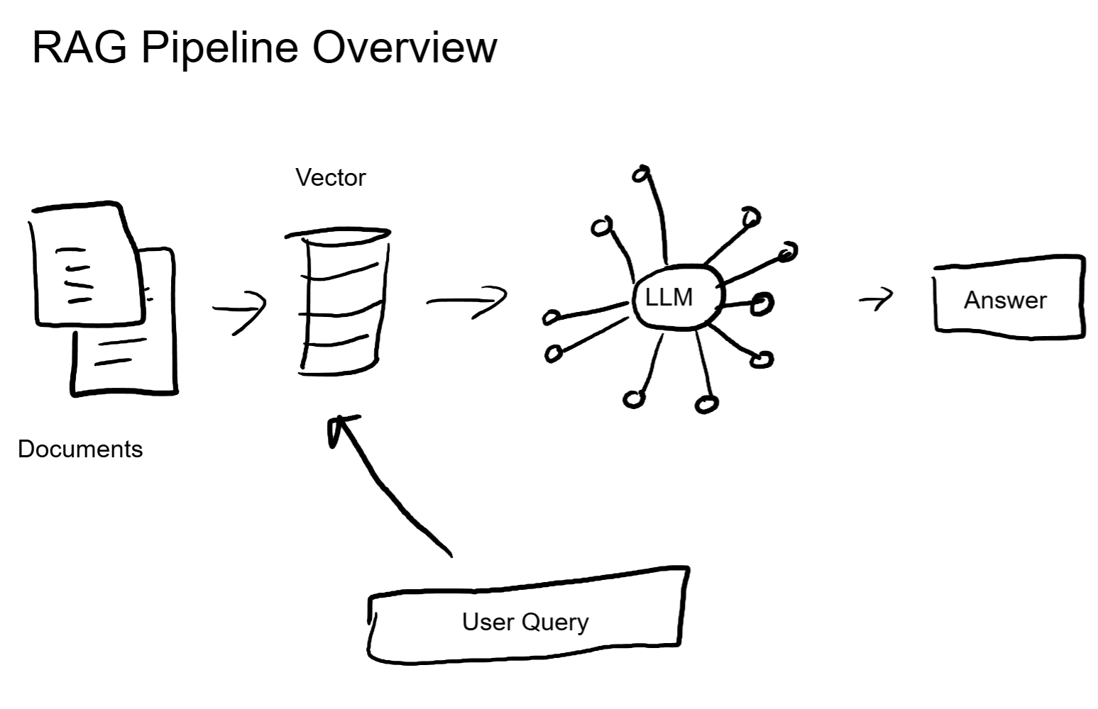
The RAG Pipeline, Step by Step

Step 1: Ingestion. Turning Documents into Something Searchable

Before an LLM can reference your data, that data needs to be broken into smaller pieces called chunks. A 200-page PDF is not useful as a single block. The model's context window has a finite size, and stuffing an entire document in there wastes space and drowns out the relevant parts.

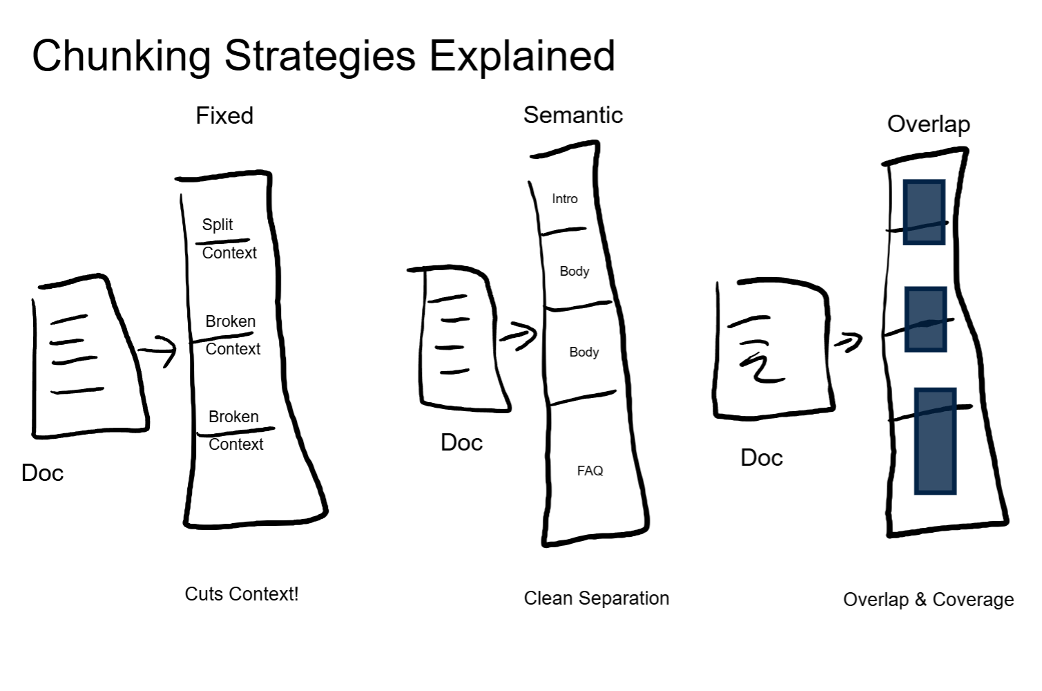
Chunking is the process of splitting documents into segments that are small enough to be useful but large enough to retain meaning. There are a few strategies:

• Fixed-size chunking splits by a set number of tokens (say, 512). Simple and predictable, but it will cut sentences and ideas in half without caring.
• Semantic chunking splits at natural boundaries: paragraph breaks, section headers, topic shifts. The chunks are variable-length but each one represents a coherent idea.
• Overlapping chunks add a buffer zone. Each chunk shares some content with the one before it and the one after it. This reduces the chance that a key piece of context lands exactly on a boundary and gets lost.

The choice here matters more than most people expect. Bad chunking is the single most common source of bad retrieval. If the system retrieves the wrong chunks, the model generates answers grounded in the wrong evidence. Garbage in, garbage out, and it starts right here.

For a business building a customer-facing agent, this is a direct quality lever. The difference between "the agent answered correctly" and "the agent hallucinated confidently" often comes down to how the source documents were split.

Step 2: Embedding. From Words to Numbers

Once the document is chunked, each chunk needs to be converted into a format a machine can compare mathematically. That format is a vector embedding: a list of numbers (typically 768 to 1536 of them) that represents the meaning of that chunk.

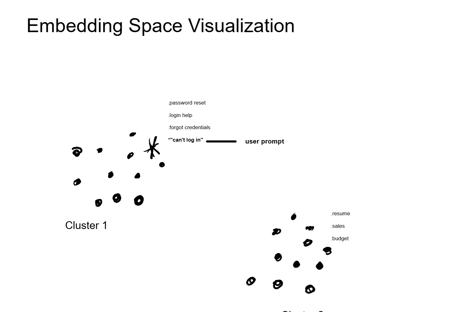
The key concept here is that the embedding captures semantics, not just keywords. The phrases "how to reset my password" and "I forgot my login credentials" look different as text, but their embeddings will be nearly identical because they mean the same thing. The embedding model learns these relationships during its own training process.

This is what makes RAG fundamentally different from old-school keyword search. A traditional search engine needs an exact or near-exact word match. Embedding-based retrieval finds content based on what it means, regardless of how it is worded.

These embedding models are separate from the LLM itself. They are smaller, faster, and purpose-built for one job: turning text into numerical representations. The LLM handles the generation. The embedding model handles the search. Two different tools, two different roles.

For anyone building a production system, this separation matters. Your embedding model runs on every document at ingestion time and on every user query at request time. Its speed and accuracy directly affect your system's latency and retrieval quality. That is a real infrastructure decision with cost implications.

Step 3: Storage. The Vector Database

All those embeddings need to live somewhere they can be searched efficiently. A traditional relational database is built for exact lookups: give me the row where id = 42. Vector databases are built for similarity lookups: give me the 10 embeddings closest to this query embedding.

That is a fundamentally different operation. Under the hood, vector databases use specialized indexing algorithms (HNSW, IVF, and others) that organize embeddings in a way that makes nearest-neighbor search fast, even across millions of vectors.

The tooling landscape here includes purpose-built vector databases like Pinecone and Weaviate, vector extensions on existing databases like pgvector for PostgreSQL, and lightweight in-memory options like Chroma for prototyping. The right choice depends on your scale, latency requirements, and existing infrastructure. This is not a product recommendation; it is just context for what exists.

From an architecture perspective, the vector database is the knowledge backbone of your RAG system. If it is slow, your agent is slow. If it is down, your agent cannot access any grounded knowledge. Treat it with the same seriousness you would give any production data store.

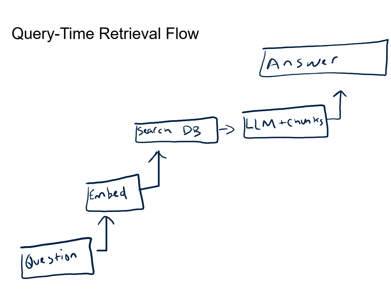
Step 4: Retrieval. Finding What Is Relevant

When a user asks a question, that question goes through the same embedding model. The query becomes a vector, just like the document chunks.

Now the system performs a similarity search. It compares the query vector against every stored chunk vector and returns the top-K results, where K is a configurable number (typically 3 to 10). The comparison uses a distance metric, most commonly cosine similarity, which measures the angle between two vectors. Small angle means similar meaning. Large angle means unrelated.

Here is the key part. The system is not doing keyword matching. It is measuring the mathematical distance between ideas. A query about "reducing inference costs" will surface chunks about "GPU memory optimization" and "batching strategies" even if those chunks never contain the word "cost." That is the power of semantic retrieval.

The top-K parameter is a real engineering decision. Too few results and the model lacks context. Too many and you waste context window space on marginally relevant content, pushing out room for the model's actual reasoning. Every production RAG system I've worked on involved tuning this number against real user queries.

Step 5: Generation. Grounded Answers

The retrieved chunks get assembled into the LLM's context window alongside the original user question and any system-level instructions. The model now generates a response with evidence sitting right in front of it.

This is the difference between a model pulling from vague training memory and a model working from specific, sourced material. The response is grounded. You can trace exactly which documents contributed to the answer. If the answer is wrong, you can look at the retrieved chunks and diagnose whether the issue was a retrieval problem (wrong chunks surfaced) or a generation problem (right chunks, but the model misinterpreted them).

That traceability is a significant deal for enterprise deployment. When a VP asks "why did the agent tell a customer X?" you need an answer better than "the neural network decided." RAG gives you that answer. You can point to the exact document, the exact passage, and the exact retrieval score that drove the response.

This is also why RAG reduces hallucination, though it does not eliminate it entirely. The model is far less likely to fabricate information when it has relevant source material in its context. But if the retrieved chunks are irrelevant or contradictory, the model can still generate a confident-sounding wrong answer. The quality of the retrieval step is everything.

Why This Matters for Real Systems

Three reasons this architecture shows up in virtually every production AI deployment:

Accuracy. The model answers from your data, not from its training corpus. Your company's return policy, your product specifications, your internal procedures. The answer reflects what is actually true for your organization.

Freshness. When a document changes, you re-chunk and re-embed it. The next query picks up the updated version. No retraining, no fine-tuning, no waiting weeks for a model refresh. For fast-moving businesses, this is the only viable approach.

Auditability. Every answer comes with receipts. You know which documents were retrieved, what their relevance scores were, and what content the model had available when it generated the response. For regulated industries, compliance teams, and anyone who needs to defend an AI-generated answer, this is non-negotiable.

This pattern shows up in every production AI system I've architected. The specific components change (different vector databases, different embedding models, different chunking strategies) but the RAG pattern itself is the constant.

The Networking Angle

If you have a networking background, RAG maps cleanly to a concept you already understand: DNS resolution.

An LLM without RAG is like a router with only static routes. It knows what was programmed into it at training time. If the destination was not in the training data, it either drops the packet (refuses to answer) or sends it to a black hole (hallucinates).

RAG adds a DNS-style lookup. At query time, the system consults an authoritative source (the vector database) to resolve the answer. The model does not need to memorize every piece of knowledge any more than a router needs to memorize every IP address. It just needs to know where to look.

And just like DNS, the quality of your authoritative source determines the quality of your responses. Stale zone files give you stale answers. A misconfigured vector database gives you irrelevant retrieval. The architecture pattern is the same; the domain is different.

What RAG Does Not Solve

RAG is foundational, but it is not a silver bullet. A few things it does not fix on its own:

Bad source data. If your documents are outdated, poorly written, or contradictory, RAG will faithfully retrieve that bad information and the model will generate answers based on it. The system is only as good as the knowledge base behind it.

Context window limits. Every retrieved chunk takes up space in the model's context window. A context window is finite, and as conversations get longer or more chunks get injected, you start competing for space. Later posts in this series cover KV cache and memory architectures that address this directly.

Retrieval latency. The embedding step and similarity search add time to every request. For real-time, high-throughput systems, this latency needs to be measured and optimized. The vector database choice, the index type, and the number of vectors all factor in.

Multi-hop reasoning. If answering a question requires combining information from multiple unrelated documents in sequence (find fact A, use it to look up fact B, combine them for the answer), basic RAG struggles. More advanced patterns like agentic RAG handle this, but that is a different architecture layer.

These are not reasons to avoid RAG. They are reasons to implement it with your eyes open and your architecture planned.

Key Takeaways

• RAG is retrieve, then generate. The LLM does not memorize your data. It receives relevant information at query time and generates a grounded response from it.
• Embeddings are the bridge. They convert human language into numerical vectors that machines can compare by meaning, not by keyword match. This is what makes semantic retrieval work.
• The LLM is the writer, not the librarian. A separate retrieval system finds the right information. The LLM's job is to synthesize it into a coherent, useful answer.
• Chunking quality drives everything downstream. The most common RAG failures trace back to how the source documents were split. Get this step right and the rest of the pipeline benefits.
• Auditability is the enterprise unlock. Being able to trace every answer back to its source documents is what separates a demo from a production deployment.

Up Next

Now that you understand how LLMs access external knowledge, the natural question is: what is actually happening inside the infrastructure when you hit send? The next post covers the hardware and engineering behind inference: GPUs, model sizes, context windows, and the four tradeoffs that define every production deployment.